
Python:PyTorch 训练网络 (七十七)
将学习条件/损失、优化器,并且如何用MNIST 训练 FF 网络的代码。
训练神经网络
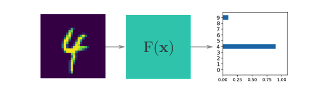
我们在上个部分构建的神经网络了解的信息很少,它不知道关于我们的手写数字的任何信息。具有非线性激活函数的神经网络就像通用函数逼近器一样。某些函数会将输入映射到输出。例如,将手写数字图像映射到类别概率。神经网络的强大之处是我们可以训练网络以逼近这个函数,基本上只要提供充足的数据和计算时间,任何函数都可以逼近。
一开始网络很朴素,不知道将输入映射到输出的函数。我们通过向网络展示实际数据样本训练网络,然后调整网络参数,使其逼近此函数。
要找到这些参数,我们需要了解网络预测真实输出的效果如何。为此,我们将计算损失函数(也称为成本),一种衡量预测错误的指标。例如,回归问题和二元分类问题经常使用均方损失
$$
\ell = \frac{1}{2n}\sum_i^n{\left(y_i - \hat{y}_i\right)^2}
$$
其中 $n$ 是训练样本的数量,$y_i$ 是真正的标签,$\hat{y}_i$ 是预测标签。
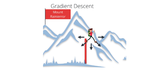
通过尽量减小相对于网络参数的这一损失,我们可以找到损失最低且网络能够以很高的准确率预测正确标签的配置。我们使用叫做梯度下降法的流程来寻找这一最低值。梯度是损失函数的斜率,指向变化最快的方向。要以最短的时间找到最低值,我们需要沿着梯度(向下)前进。可以将这一过程看做沿着最陡的路线下山。
反向传播
对于单层网络,梯度下降法实现起来很简单。但是,对于更深、层级更多的神经网络(例如我们构建的网络),梯度下降法实现起来更复杂,以至于需要大约 30 年时间研究人员才能弄明白如何训练多层网络,虽然了解这一概念后会发现很简单。
我们通过反向传播来实现,实际上是采用的微积分中的链式法则。最简单的理解方法是将两层网络转换为图形表示法。
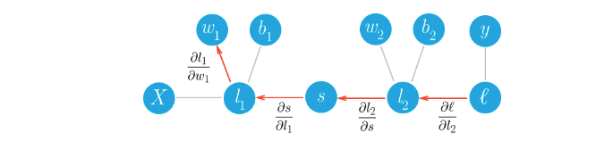
在网络的前向传递过程中,我们的数据和运算从左到右。要通过梯度下降法训练权重,我们沿着网络反向传播成本梯度。从数学角度来讲,其实就是使用链式法则计算相对于权重的损失梯度。
$$
\frac{\partial \ell}{\partial w_1} = \frac{\partial l_1}{\partial w_1} \frac{\partial s}{\partial l_1} \frac{\partial l_2}{\partial s} \frac{\partial \ell}{\partial l_2}
$$
我们使用此梯度和学习速率 $\alpha$ 更新权重。
$$
w^\prime = w - \alpha \frac{\partial \ell}{\partial w}
$$
设置学习速率的方式是权重更新步长很小,使迭代方法能达到最小值。
对于训练步骤来说,首先我们需要定义损失函数。在 PyTorch 中,通常你会看到它写成了 criterion 形式。在此例中,我们使用 softmax 输出,因此我们希望使用 criterion = nn.CrossEntropyLoss() 作为损失函数。稍后在训练时,你需要使用 loss = criterion(output, targets) 计算实际损失。
我们还需要定义优化器,例如 SGD 或 Adam 等。我将使用 SGD,即 torch.optim.SGD,并传入网络参数和学习速率。
Autograd
Torch 提供了模块 autograd 用于自动计算张量的梯度。计算方式是跟踪在张量上执行的运算。要让 PyTorch 跟踪运算,你需要使用 torch.autograd 的 Variable 类封装张量。你可以使用 Variable 的 .data 属性获取张量。
我们使用 z.backward() 计算相对于变量 z 的梯度。这样会对创建 z 的运算进行反向传递。
%matplotlib inline
%config InlineBackend.figure_format = 'retina'

import numpy as np
import time

import torch
from torch import nn
from torch import optim
import torch.nn.functional as F
from torch.autograd import Variable

import helper
x = torch.randn(2,2)
x = Variable(x, requires_grad=True)
print(x)tensor([[ 2.0177, -1.4438],
[-0.8740, 1.4361]])y = x**2
print(y)tensor([[ 4.0712, 2.0845],
[ 0.7639, 2.0623]])我们可以在下面看到创建 y 的运算,即幂运算 PowBackward0.
## grad_fn shows the function that generated this variable
print(y.grad_fn)
<PowBackward0 object at 0x7fc13410ba90>autgrad 模块会跟踪这些运算并知道如何为每个运算计算梯度。这样的话,它就能够计算一系列运算相对于任何一个张量的梯度。我们将张量 y 简化为标量值,即均值。
z = y.mean()
print(z)tensor(2.2455)你可以查看 x 和 y 的梯度,但是现在它们为空。
print(x.grad)None要计算梯度,你需要对 Variable(例如 z)运行 .backward 方法。这样会计算 z 相对于 x 的梯度
$$
\frac{\partial z}{\partial x} = \frac{\partial}{\partial x}\left[\frac{1}{n}\sum_i^n x_i^2\right] = \frac{x}{2}
$$
z.backward()
print(x.grad)
print(x/2)
tensor([[ 1.0089, -0.7219],
[-0.4370, 0.7180]])
tensor([[ 1.0089, -0.7219],
[-0.4370, 0.7180]])这些梯度运算对神经网络来说尤其有用。对于训练来说,我们需要得出权重相对于成本的梯度。对于 PyTorch,我们在网络中向前运行数据以计算成本,然后向后传播以计算相对于成本的梯度。得出梯度后,我们可以执行梯度下降步。
训练网络!
对于训练步骤来说,首先我们需要定义损失函数。在 PyTorch 中,通常你会看到它写成了 criterion 形式。在此例中,我们使用 softmax 输出,因此我们希望使用 criterion = nn.CrossEntropyLoss() 作为损失函数。稍后在训练时,你需要使用 loss = criterion(output, targets) 计算实际损失。
我们还需要定义优化器,例如 SGD 或 Adam 等。我将使用 SGD,即 torch.optim.SGD,并传入网络参数和学习速率。
from torchvision import datasets, transforms

# Define a transform to normalize the data
transform = transforms.Compose([transforms.ToTensor(),
                              transforms.Normalize((0.5, 0.5, 0.5), (0.5, 0.5, 0.5)),
                             ])
# Download and load the training data
trainset = datasets.MNIST('MNIST_data/', download=True, train=True, transform=transform)
trainloader = torch.utils.data.DataLoader(trainset, batch_size=64, shuffle=True)

# Download and load the test data
testset = datasets.MNIST('MNIST_data/', download=True, train=False, transform=transform)
testloader = torch.utils.data.DataLoader(testset, batch_size=64, shuffle=True)
class Network(nn.Module):
def __init__(self):
super().__init__()
# Defining the layers, 200, 50, 10 units each
self.fc1 = nn.Linear(784, 200)
self.fc2 = nn.Linear(200, 50)
# Output layer, 10 units - one for each digit
self.fc3 = nn.Linear(50, 10)
def forward(self, x):
''' Forward pass through the network, returns the output logits '''
x = self.fc1(x)
x = F.relu(x)
x = self.fc2(x)
x = F.relu(x)
x = self.fc3(x)
return x
def predict(self, x):
''' This function for predicts classes by calculating the softmax '''
logits = self.forward(x)
return F.softmax(logits, dim=1)net = Network()
criterion = nn.CrossEntropyLoss()
optimizer = optim.SGD(net.parameters(), lr=0.01)首先我们只考虑一个学习步,然后再循环访问所有数据。PyTorch 的一般流程是:
- 在网络中进行前向传递以获得 logits
- 使用 logits 计算损失
- 通过
loss.backward()对网络进行反向传递以计算梯度 - 用优化器执行一步以更新权重
我将在下面完成一个训练步并输出权重和梯度,使你能够明白变化过程。
rint('print fc1 - ', net.fc1)

print('Initial weights - ', net.fc1.weight)

print('print trainloader- ', trainloader)
dataiter = iter(trainloader)

print('print dataiter- ', dataiter)

images, labels = dataiter.next()

print('print images- ', images)
print('print labels- ', labels)

images.resize_(64, 784)

# Create Variables for the inputs and targets
inputs = Variable(images)
targets = Variable(labels)

print('print inputs:', inputs)

# Clear the gradients from all Variables
optimizer.zero_grad()

# Forward pass, then backward pass, then update weights
output = net.forward(inputs)
loss = criterion(output, targets)
loss.backward()
print('Gradient -', net.fc1.weight.grad)
optimizer.step()
print fc1 - Linear(in_features=784, out_features=200, bias=True)
Initial weights - Parameter containing:
tensor([[ 8.5397e-03, 2.0490e-02, -3.0762e-02, ..., 2.7010e-02,
1.2961e-02, 6.6650e-03],
[ 2.4989e-02, -2.4855e-02, -1.3049e-02, ..., -3.4125e-03,
-1.0886e-03, -2.1010e-03],
[ 2.5357e-02, -7.1994e-04, 2.0392e-02, ..., 1.1883e-02,
-3.0476e-02, -1.7069e-02],
...,
[ 2.9283e-02, 1.7928e-02, -1.9773e-03, ..., 9.2352e-03,
1.9706e-02, -6.5281e-03],
[ 4.0206e-02, 1.8597e-02, -5.2074e-03, ..., 3.0402e-02,
8.5699e-03, 2.0727e-02],
[ 8.6584e-03, 1.3021e-03, 9.7864e-03, ..., 1.1017e-02,
-2.7003e-02, 2.3624e-02]])
print trainloader- <torch.utils.data.dataloader.DataLoader object at 0x7f7b281599b0>
print dataiter- <torch.utils.data.dataloader._DataLoaderIter object at 0x7f7b2361ff60>
print images- tensor([[[[-1.0000, -1.0000, -1.0000, ..., -1.0000, -1.0000, -1.0000],
[-1.0000, -1.0000, -1.0000, ..., -1.0000, -1.0000, -1.0000],
[-1.0000, -1.0000, -1.0000, ..., -1.0000, -1.0000, -1.0000],
...,
[-1.0000, -1.0000, -1.0000, ..., -1.0000, -1.0000, -1.0000],
[-1.0000, -1.0000, -1.0000, ..., -1.0000, -1.0000, -1.0000],
[-1.0000, -1.0000, -1.0000, ..., -1.0000, -1.0000, -1.0000]]],
[[[-1.0000, -1.0000, -1.0000, ..., -1.0000, -1.0000, -1.0000],
[-1.0000, -1.0000, -1.0000, ..., -1.0000, -1.0000, -1.0000],
[-1.0000, -1.0000, -1.0000, ..., -1.0000, -1.0000, -1.0000],
...,
[-1.0000, -1.0000, -1.0000, ..., -1.0000, -1.0000, -1.0000],
[-1.0000, -1.0000, -1.0000, ..., -1.0000, -1.0000, -1.0000],
[-1.0000, -1.0000, -1.0000, ..., -1.0000, -1.0000, -1.0000]]],
...,
[[[-1.0000, -1.0000, -1.0000, ..., -1.0000, -1.0000, -1.0000],
[-1.0000, -1.0000, -1.0000, ..., -1.0000, -1.0000, -1.0000],
[-1.0000, -1.0000, -1.0000, ..., -1.0000, -1.0000, -1.0000],
...,
[-1.0000, -1.0000, -1.0000, ..., -1.0000, -1.0000, -1.0000],
[-1.0000, -1.0000, -1.0000, ..., -1.0000, -1.0000, -1.0000],
[-1.0000, -1.0000, -1.0000, ..., -1.0000, -1.0000, -1.0000]]],
[[[-1.0000, -1.0000, -1.0000, ..., -1.0000, -1.0000, -1.0000],
[-1.0000, -1.0000, -1.0000, ..., -1.0000, -1.0000, -1.0000],
[-1.0000, -1.0000, -1.0000, ..., -1.0000, -1.0000, -1.0000],
...,
[-1.0000, -1.0000, -1.0000, ..., -1.0000, -1.0000, -1.0000],
[-1.0000, -1.0000, -1.0000, ..., -1.0000, -1.0000, -1.0000],
[-1.0000, -1.0000, -1.0000, ..., -1.0000, -1.0000, -1.0000]]]])
print labels- tensor([ 0, 0, 4, 6, 0, 7, 3, 3, 4, 3, 6, 3, 8, 1,
2, 5, 5, 4, 3, 2, 8, 7, 1, 8, 2, 5, 3, 0,
8, 3, 5, 8, 2, 0, 8, 0, 6, 9, 1, 7, 4, 5,
8, 0, 1, 1, 7, 3, 7, 6, 9, 9, 6, 7, 0, 9,
3, 7, 9, 9, 3, 2, 0, 8])
print inputs: tensor([[-1.0000, -1.0000, -1.0000, ..., -1.0000, -1.0000, -1.0000],
[-1.0000, -1.0000, -1.0000, ..., -1.0000, -1.0000, -1.0000],
[-1.0000, -1.0000, -1.0000, ..., -1.0000, -1.0000, -1.0000],
...,
[-1.0000, -1.0000, -1.0000, ..., -1.0000, -1.0000, -1.0000],
[-1.0000, -1.0000, -1.0000, ..., -1.0000, -1.0000, -1.0000],
[-1.0000, -1.0000, -1.0000, ..., -1.0000, -1.0000, -1.0000]])
Gradient - tensor(1.00000e-03 *
[[-0.9912, -0.9912, -0.9912, ..., -0.9912, -0.9912, -0.9912],
[ 0.0000, 0.0000, 0.0000, ..., 0.0000, 0.0000, 0.0000],
[ 1.7549, 1.7549, 1.7549, ..., 1.7549, 1.7549, 1.7549],
...,
[ 0.0000, 0.0000, 0.0000, ..., 0.0000, 0.0000, 0.0000],
[ 0.0000, 0.0000, 0.0000, ..., 0.0000, 0.0000, 0.0000],
[ 0.0000, 0.0000, 0.0000, ..., 0.0000, 0.0000, 0.0000]])print('Updated weights - ', net.fc1.weight)Updated weights - Parameter containing:
tensor([[-2.3054e-02, -7.3247e-03, 3.3989e-02, ..., 1.4626e-03,
-2.4275e-04, 2.5772e-02],
[-1.4883e-02, -6.8011e-03, 1.4760e-02, ..., 2.2036e-02,
8.5643e-03, 3.2226e-02],
[-1.3967e-02, -7.4284e-05, -3.3173e-02, ..., 2.1535e-02,
2.9550e-02, -2.5174e-02],
...,
[ 4.2445e-03, 1.3663e-02, 1.1734e-02, ..., 3.2027e-02,
-3.1084e-03, 2.8480e-02],
[ 2.3525e-02, 1.5927e-02, -2.5106e-02, ..., -1.0978e-02,
-1.4049e-02, 9.7510e-03],
[-2.5424e-02, -3.7520e-03, 3.4995e-02, ..., 1.8272e-02,
-6.4011e-03, -1.3063e-02]])实际训练
现在,我们将此算法用于循环中,以便访问所有图像。很简单,我们将循环访问数据集的小批次数据,在网络中传递数据以计算损失,获得梯度,然后运行优化器。
net = Network()
optimizer = optim.Adam(net.parameters(), lr=0.001)
epochs = 1
steps = 0
running_loss = 0
print_every = 20
for e in range(epochs):
for images, labels in iter(trainloader):
steps += 1
# Flatten MNIST images into a 784 long vector
images.resize_(images.size()[0], 784)
# Wrap images and labels in Variables so we can calculate gradients
inputs = Variable(images)
targets = Variable(labels)
optimizer.zero_grad()
output = net.forward(inputs)
loss = criterion(output, targets)
loss.backward()
optimizer.step()
running_loss += loss.data[0]
if steps % print_every == 0:
# Test accuracy
accuracy = 0
for ii, (images, labels) in enumerate(testloader):
images = images.resize_(images.size()[0], 784)
inputs = Variable(images, volatile=True)
predicted = net.predict(inputs).data
equality = (labels == predicted.max(1)[1])
accuracy += equality.type_as(torch.FloatTensor()).mean()
print("Epoch: {}/{}".format(e+1, epochs),
"Loss: {:.4f}".format(running_loss/print_every),
"Test accuracy: {:.4f}".format(accuracy/(ii+1)))
running_loss = 0/opt/conda/lib/python3.6/site-packages/ipykernel_launcher.py:21: UserWarning: invalid index of a 0-dim tensor. This will be an error in PyTorch 0.5. Use tensor.item() to convert a 0-dim tensor to a Python number
/opt/conda/lib/python3.6/site-packages/ipykernel_launcher.py:29: UserWarning: volatile was removed and now has no effect. Use `with torch.no_grad():` instead.
Epoch: 1/1 Loss: 1.9097 Test accuracy: 0.6854
Epoch: 1/1 Loss: 1.1061 Test accuracy: 0.7751
Epoch: 1/1 Loss: 0.7042 Test accuracy: 0.8204
Epoch: 1/1 Loss: 0.5564 Test accuracy: 0.8457
Epoch: 1/1 Loss: 0.5339 Test accuracy: 0.8407
Epoch: 1/1 Loss: 0.5396 Test accuracy: 0.8608
Epoch: 1/1 Loss: 0.4474 Test accuracy: 0.8873
Epoch: 1/1 Loss: 0.4038 Test accuracy: 0.8887
Epoch: 1/1 Loss: 0.4636 Test accuracy: 0.8880
Epoch: 1/1 Loss: 0.3866 Test accuracy: 0.8908
Epoch: 1/1 Loss: 0.4189 Test accuracy: 0.8814
Epoch: 1/1 Loss: 0.4408 Test accuracy: 0.8911
Epoch: 1/1 Loss: 0.3593 Test accuracy: 0.8952
Epoch: 1/1 Loss: 0.3571 Test accuracy: 0.8991
Epoch: 1/1 Loss: 0.3540 Test accuracy: 0.8888
Epoch: 1/1 Loss: 0.3815 Test accuracy: 0.8910
Epoch: 1/1 Loss: 0.3729 Test accuracy: 0.8936
Epoch: 1/1 Loss: 0.3273 Test accuracy: 0.9001
Epoch: 1/1 Loss: 0.3517 Test accuracy: 0.8982
Epoch: 1/1 Loss: 0.3505 Test accuracy: 0.8962
Epoch: 1/1 Loss: 0.3411 Test accuracy: 0.8982
Epoch: 1/1 Loss: 0.3639 Test accuracy: 0.9171
Epoch: 1/1 Loss: 0.3541 Test accuracy: 0.9149
Epoch: 1/1 Loss: 0.3050 Test accuracy: 0.9155
Epoch: 1/1 Loss: 0.3200 Test accuracy: 0.9138
Epoch: 1/1 Loss: 0.3314 Test accuracy: 0.9111
Epoch: 1/1 Loss: 0.2506 Test accuracy: 0.9157
Epoch: 1/1 Loss: 0.2568 Test accuracy: 0.9113
Epoch: 1/1 Loss: 0.3099 Test accuracy: 0.9148
Epoch: 1/1 Loss: 0.2746 Test accuracy: 0.9104
Epoch: 1/1 Loss: 0.2986 Test accuracy: 0.9194
Epoch: 1/1 Loss: 0.2738 Test accuracy: 0.9274
Epoch: 1/1 Loss: 0.2576 Test accuracy: 0.9203
Epoch: 1/1 Loss: 0.2592 Test accuracy: 0.9209
Epoch: 1/1 Loss: 0.3085 Test accuracy: 0.9219
Epoch: 1/1 Loss: 0.3040 Test accuracy: 0.9235
Epoch: 1/1 Loss: 0.2466 Test accuracy: 0.9258
Epoch: 1/1 Loss: 0.2511 Test accuracy: 0.9258
Epoch: 1/1 Loss: 0.2586 Test accuracy: 0.9277
Epoch: 1/1 Loss: 0.2779 Test accuracy: 0.9274
Epoch: 1/1 Loss: 0.2639 Test accuracy: 0.9360
Epoch: 1/1 Loss: 0.2621 Test accuracy: 0.9376
Epoch: 1/1 Loss: 0.2230 Test accuracy: 0.9340
Epoch: 1/1 Loss: 0.2481 Test accuracy: 0.9322
Epoch: 1/1 Loss: 0.1941 Test accuracy: 0.9416
Epoch: 1/1 Loss: 0.2000 Test accuracy: 0.9406dataiter = iter(testloader)
images, labels = dataiter.next()img = images[0]
ps = net.predict(Variable(img.resize_(1, 784)))
helper.view_classify(img.resize_(1, 28, 28), ps)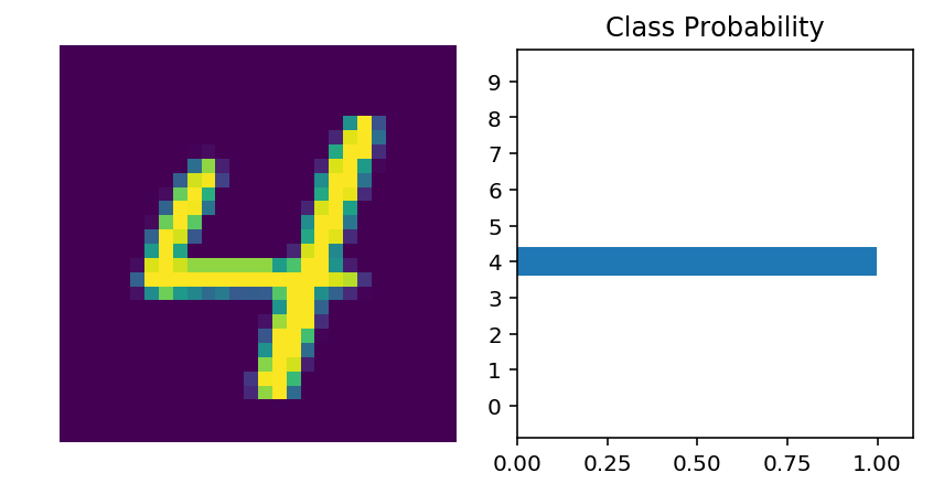
我们的网络现在并不是一无所知了。它可以准确地预测图像中的数字。接着,你将编写用更复杂的数据集训练神经网络的代码。
为者常成,行者常至
自由转载-非商用-非衍生-保持署名(创意共享3.0许可证)


