AI For Trading:Smoothing (66)

Smoothing

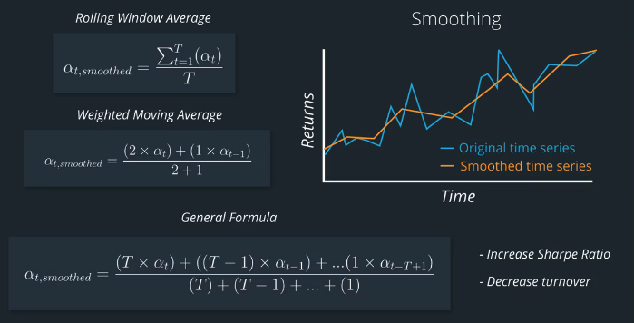
Financial data is noisy, and sometimes the data we're working with is sparse. For instance, it might have many missing values. We can apply smoothing techniques across the time dimension to help make the factor more robust to noise and sparse data.

Quize

Check out the documentation for two smoothing functions: simplemovingaverage and exponentialWeightedMovingAverage

练习题

How would you set the arguments of the ExponentialWeightedMovingAverage so that it gave the same result as SimpleMovingAverage?

A：decay=SimpleMovingAverage
B: decay=0
C: decay=1
D: decay = NaN

答案：C

Smoothing

Install packages

import sys

!{sys.executable} -m pip install -r requirements.txt

import cvxpy as cvx
import numpy as np
import pandas as pd
import time
import os
import quiz_helper
import matplotlib.pyplot as plt

%matplotlib inline
plt.style.use('ggplot')
plt.rcParams['figure.figsize'] = (14, 8)

data bundle

import os
import quiz_helper
from zipline.data import bundles

os.environ['ZIPLINE_ROOT'] = os.path.join(os.getcwd(), '..', '..','data','module_4_quizzes_eod')
ingest_func = bundles.csvdir.csvdir_equities(['daily'], quiz_helper.EOD_BUNDLE_NAME)
bundles.register(quiz_helper.EOD_BUNDLE_NAME, ingest_func)
print('Data Registered')

Build pipeline engine

from zipline.pipeline import Pipeline
from zipline.pipeline.factors import AverageDollarVolume
from zipline.utils.calendars import get_calendar

universe = AverageDollarVolume(window_length=120).top(500) 
trading_calendar = get_calendar('NYSE') 
bundle_data = bundles.load(quiz_helper.EOD_BUNDLE_NAME)
engine = quiz_helper.build_pipeline_engine(bundle_data, trading_calendar)

View Data露

With the pipeline engine built, let's get the stocks at the end of the period in the universe we're using. We'll use these tickers to generate the returns data for the our risk model.

universe_end_date = pd.Timestamp('2016-01-05', tz='UTC')

universe_tickers = engine\
    .run_pipeline(
        Pipeline(screen=universe),
        universe_end_date,
        universe_end_date)\
    .index.get_level_values(1)\
    .values.tolist()

universe_tickers

Get Returns data

from zipline.data.data_portal import DataPortal

data_portal = DataPortal(
    bundle_data.asset_finder,
    trading_calendar=trading_calendar,
    first_trading_day=bundle_data.equity_daily_bar_reader.first_trading_day,
    equity_minute_reader=None,
    equity_daily_reader=bundle_data.equity_daily_bar_reader,
    adjustment_reader=bundle_data.adjustment_reader)

Get pricing data helper function

def get_pricing(data_portal, trading_calendar, assets, start_date, end_date, field='close'):
    end_dt = pd.Timestamp(end_date.strftime('%Y-%m-%d'), tz='UTC', offset='C')
    start_dt = pd.Timestamp(start_date.strftime('%Y-%m-%d'), tz='UTC', offset='C')

    end_loc = trading_calendar.closes.index.get_loc(end_dt)
    start_loc = trading_calendar.closes.index.get_loc(start_dt)

    return data_portal.get_history_window(
        assets=assets,
        end_dt=end_dt,
        bar_count=end_loc - start_loc,
        frequency='1d',
        field=field,
        data_frequency='daily')

get pricing data into a dataframe

returns_df = \
    get_pricing(
        data_portal,
        trading_calendar,
        universe_tickers,
        universe_end_date - pd.DateOffset(years=5),
        universe_end_date)\
    .pct_change()[1:].fillna(0) #convert prices into returns

returns_df

Sector data helper function

We'll create an object for you, which defines a sector for each stock. The sectors are represented by integers. We inherit from the Classifier class. Documentation for Classifier, and the source code for Classifier

from zipline.pipeline.classifiers import Classifier
from zipline.utils.numpy_utils import int64_dtype
class Sector(Classifier):
    dtype = int64_dtype
    window_length = 0
    inputs = ()
    missing_value = -1

    def __init__(self):
        self.data = np.load('../../data/project_4_sector/data.npy')

    def _compute(self, arrays, dates, assets, mask):
        return np.where(
            mask,
            self.data[assets],
            self.missing_value,
        )

sector = Sector()

We'll use 2 years of data to calculate the factor

Note: Going back 2 years falls on a day when the market is closed. Pipeline package doesn't handle start or end dates that don't fall on days when the market is open. To fix this, we went back 2 extra days to fall on the next day when the market is open.

factor_start_date = universe_end_date - pd.DateOffset(years=2, days=2)
factor_start_date

Explore the SimpleMovingAverage Function

The documentation for SimpleMovingAverage is located here, and is also pasted below:

class zipline.pipeline.factors.SimpleMovingAverage(*args, **kwargs)[source]
Average Value of an arbitrary column

Default Inputs: None

Default Window Length: None

Notice that the description doesn't show us the syntax for the parameters for Inputs and Window Length. Looking at the source code, we can see that SimpleMovingAverage is a class that inherits from CustomFactor.

Here's the documentation for CustomFactor. Notice that it includes parameters inputs and window_length.

Quiz 1

Create a factor of one year returns, demeaned, and ranked, and then converted to a zscore.

Put this factor as the input into a SimpleMovingAverage function, with a window length for 1 week (5 trading days). Also rank and zscore this smoothed factor. Note that you don't need to make it sector neutral, since the original factor is already demeaned by sector.

Answer 1

#TODO: import Returns from zipline
from zipline.pipeline.factors import Returns
# TODO: import SimpleMovingAverage from zipline
from zipline.pipeline.factors import SimpleMovingAverage

#TODO
# create a pipeline called p
p = Pipeline(screen=universe)
# create a factor of one year returns, deman by sector, then rank
factor = (
    Returns(window_length=252, mask=universe).
    demean(groupby=Sector()). #we use the custom Sector class that we reviewed earlier
    rank().
    zscore()
)

# TODO
# Use this factor as input into SimpleMovingAverage, with a window length of 5
# Also rank and zscore (don't need to de-mean by sector, s)
factor_smoothed = (
    SimpleMovingAverage(inputs=[factor], window_length=5).
    rank().
    zscore()
)

# add the unsmoothed factor to the pipeline
p.add(factor, 'Momentum_Factor')
# add the smoothed factor to the pipeline too
p.add(factor_smoothed, 'Smoothed_Momentum_Factor')

visualize the pipeline

Note that if the image is difficult to read in the notebook, right-click and view the image in a separate tab.

p.show_graph(format='png')

run pipeline and view the factor data

df = engine.run_pipeline(p, factor_start_date, universe_end_date)

df.head()

Let's grab some data for one stock

# these are the index values for all the stocks (index level 1)
df.index.get_level_values(1)[0:5]

Quiz 2

Get the index value for APPL stock

Answer 2

# TODO
# get the level value for AAPL (it's at row index 3)
stock_index_name = df.index.get_level_values(1)[3]

print(type(stock_index_name))
print(stock_index_name)

Stack overflow example of how to use numpy.in1d

https://stackoverflow.com/questions/25224545/filtering-muliple-items-in-a-multi-index-python-panda-dataframe

#notice, we'll put the stock_index_name inside of a list
single_stock_df = df[np.in1d(df.index.get_level_values(1), [stock_index_name])]
single_stock_df.head()

single_stock_df['Momentum_Factor'].plot()
single_stock_df['Smoothed_Momentum_Factor'].plot(style='--')

Quiz 3

How would you describe the smoothed factor values compared to unsmoothed factor values?

Answer 3

The smoothed factor values follow the original factor values but are a bit less volatile (they're smoother)!

为者常成，行者常至