AI For Trading:Winners and Losers in Momentum Investing (76)

The Formation Process of Winners and Losers in Momentum Investing

Abstract:

Previous studies have focused on which stocks are winners or losers but have paid little attention to the formation process of past returns. This paper develops a model showing that past returns and the formation process of past returns have a joint effect on future expected returns. The empirical evidence shows that the zero-investment portfolio, including stocks with specific patterns of historical prices, improves monthly momentum profit by 59%. Overall, the process of how one stock becomes a winner or loser can further distinguish the best and worst stocks in a group of winners or losers.

Notes

p. 3: Intermediate-term (3–12 months) momentum has been documented by Jegadeesh and Titman (1993, 2001, hereafter JT), while short-term (weekly) and long-term (3–5 years) reversals have been documented by Lehmann (1990) and Jegadeesh (1990) and by DeBondt and Thaler (1985), respectively. Various models and theories have been proposed to explain the coexistence of intermediate-term momentum and long-term reversal. However, most studies have focused primarily on which stocks are winners or losers; they have paid little attention to how those stocks become winners or losers. This paper develops a model to analyze whether the movement of historical prices is related to future expected returns.

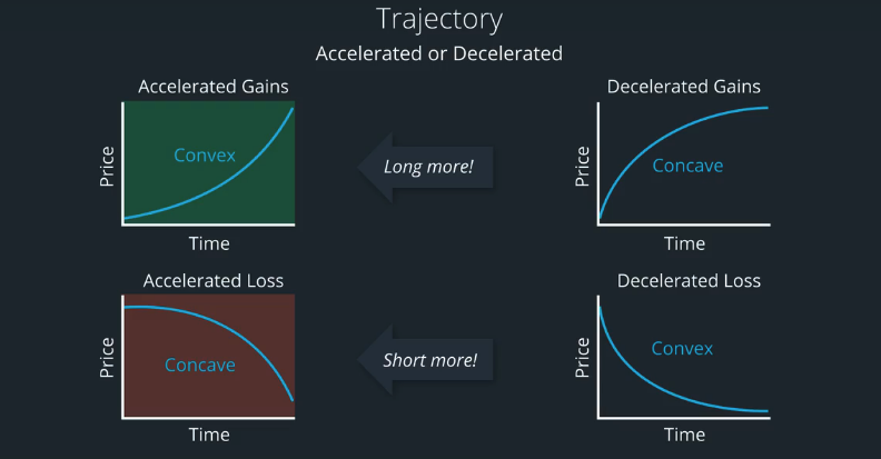
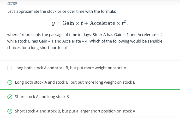
p. 4: This paper captures the idea that past returns and the formation process of past returns have a joint effect on future expected returns. We argue that how one stock becomes a winner or loser—that is, the movement of historical prices—plays an important role in momentum investing. Using a polynomial quadratic model to approximate the nonlinear pattern of historical prices, the model shows that as long as two stocks share the same return over the past n-month, the future expected return of the stock whose historical prices are convex shaped is not lower than one whose historical prices are concave shaped. In other words, when there are two winner (or loser) stocks, the one with convex-shaped historical prices will possess higher future expected returns than the one with concave-shaped historical prices.

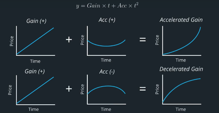
p. 4: To test the model empirically, we regress previous daily prices in the ranking period on an ordinal time variable and the square of the ordinal time variable for each stock. The coefficient of the square of the ordinal time variable is denoted as gamma.

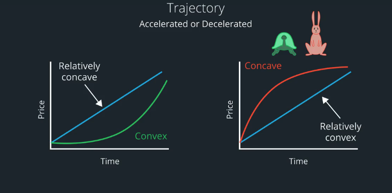
You may recall with the example of the tortoise stock and the rabbit stock. The tortoise stock trajectory looks like a straight line, whereas the rabbits stock was concave.

Winners and Losers: approximating curves with polynomials

Winners and Losers Content Quiz

Regression Against Time

The Formation Process of Winners and Losers in Momentum Investing

(https://papers.ssrn.com/sol3/papers.cfm?abstract_id=2610571)

p. 3: Intermediate-term (3–12 months) momentum has been documented by Jegadeesh
and Titman (1993, 2001, hereafter JT), while short-term (weekly) and long-term (3–5
years) reversals have been documented by Lehmann (1990) and Jegadeesh (1990) and
by DeBondt and Thaler (1985), respectively. Various models and theories have been
proposed to explain the coexistence of intermediate-term momentum and long-term
reversal. However, most studies have focused primarily on which stocks are winners
or losers; they have paid little attention to how those stocks become winners or losers.
This paper develops a model to analyze whether the movement of historical prices is
related to future expected returns.

p. 4: This paper captures the idea that past returns and the formation process of past
returns have a joint effect on future expected returns. We argue that how one stock
becomes a winner or loser—that is, the movement of historical prices—plays an
important role in momentum investing. Using a polynomial quadratic model to
approximate the nonlinear pattern of historical prices, the model shows that as long as
two stocks share the same return over the past n-month, the future expected return of
the stock whose historical prices are convex shaped is not lower than one whose
historical prices are concave shaped. In other words, when there are two winner (or
loser) stocks, the one with convex-shaped historical prices will possess higher future
expected returns than the one with concave-shaped historical prices.

p. 4: To test the model empirically, we regress previous daily prices in the ranking
period on an ordinal time variable and the square of the ordinal time variable for each
stock. The coefficient of the square of the ordinal time variable is denoted as $\gamma$.

Install packages

import sys

!{sys.executable} -m pip install -r requirements.txt

import cvxpy as cvx
import numpy as np
import pandas as pd
import time
import os
import quiz_helper
import matplotlib.pyplot as plt

%matplotlib inline
plt.style.use('ggplot')
plt.rcParams['figure.figsize'] = (14, 8)

data bundle

import os
import quiz_helper
from zipline.data import bundles

os.environ['ZIPLINE_ROOT'] = os.path.join(os.getcwd(), '..', '..','data','module_4_quizzes_eod')
ingest_func = bundles.csvdir.csvdir_equities(['daily'], quiz_helper.EOD_BUNDLE_NAME)
bundles.register(quiz_helper.EOD_BUNDLE_NAME, ingest_func)
print('Data Registered')

Build pipeline engine

from zipline.pipeline import Pipeline
from zipline.pipeline.factors import AverageDollarVolume
from zipline.utils.calendars import get_calendar

universe = AverageDollarVolume(window_length=120).top(500) 
trading_calendar = get_calendar('NYSE') 
bundle_data = bundles.load(quiz_helper.EOD_BUNDLE_NAME)
engine = quiz_helper.build_pipeline_engine(bundle_data, trading_calendar)

View Data

With the pipeline engine built, let's get the stocks at the end of the period in the universe we're using. We'll use these tickers to generate the returns data for the our risk model.

universe_end_date = pd.Timestamp('2016-01-05', tz='UTC')

universe_tickers = engine\
    .run_pipeline(
        Pipeline(screen=universe),
        universe_end_date,
        universe_end_date)\
    .index.get_level_values(1)\
    .values.tolist()

universe_tickers

Get Returns data

from zipline.data.data_portal import DataPortal

data_portal = DataPortal(
    bundle_data.asset_finder,
    trading_calendar=trading_calendar,
    first_trading_day=bundle_data.equity_daily_bar_reader.first_trading_day,
    equity_minute_reader=None,
    equity_daily_reader=bundle_data.equity_daily_bar_reader,
    adjustment_reader=bundle_data.adjustment_reader)

Get pricing data helper function

from quiz_helper import get_pricing

get pricing data into a dataframe

returns_df = \
    get_pricing(
        data_portal,
        trading_calendar,
        universe_tickers,
        universe_end_date - pd.DateOffset(years=5),
        universe_end_date)\
    .pct_change()[1:].fillna(0) #convert prices into returns

returns_df

Sector data helper function

We'll create an object for you, which defines a sector for each stock. The sectors are represented by integers. We inherit from the Classifier class. Documentation for Classifier, and the source code for Classifier

from zipline.pipeline.classifiers import Classifier
from zipline.utils.numpy_utils import int64_dtype
class Sector(Classifier):
    dtype = int64_dtype
    window_length = 0
    inputs = ()
    missing_value = -1

    def __init__(self):
        self.data = np.load('../../data/project_4_sector/data.npy')

    def _compute(self, arrays, dates, assets, mask):
        return np.where(
            mask,
            self.data[assets],
            self.missing_value,
        )

sector = Sector()

We'll use 2 years of data to calculate the factor

Note: Going back 2 years falls on a day when the market is closed. Pipeline package doesn't handle start or end dates that don't fall on days when the market is open. To fix this, we went back 2 extra days to fall on the next day when the market is open.

factor_start_date = universe_end_date - pd.DateOffset(years=2, days=2)
factor_start_date

describing price over time with a curve

To describe price over time, we'll use integers that increment each day as the independent variable. We'll use price as the dependent variable. Let's practice how to regress the stock price against time and time squared. This will allow us to describe the trajectory of price over time using a polynomial.

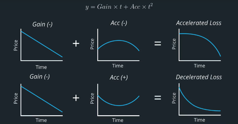
$$ ClosePrice_i = \beta \times time_i + \gamma \times time_i^2$$

First, we'll use numpy.arange(days) where days might be 5 for a week, or 252 for a year's worth of data. So we'll have integers represent the days in this window.

To create a 2D numpy array, we can combine them together in a list. By default, the numpy.arange arrays are row vectors, so we use transpose to make them column vectors (one column for each independent variable).

We instantiate a LinearRegression object, then call .fit(X,y), passing in the independent and depend variables.

We'll use .coefficient to access the coefficients estimated from the data. There is one for each independent variable.

# we're choosing a window of 5 days as an example
X = np.array([np.arange(5), np.arange(5)**2])
X = X.T
X

#we're making up some numbers to represent the stock price
y = np.array(np.random.random(5)*2)
y

from sklearn.linear_model import LinearRegression

reg = LinearRegression()
reg.fit(X,y);

Quiz 1

Output the estimates for $\beta$ and $\gamma$

# TODO Output the estimates for Beta and gamma
print(f"The beta is {reg.coef_[0]:.4f} and gamma is {reg.coef_[1]:.4f}")

outputs

outputs is a class variable defined in CustomFactor class. We'll set outputs to a list of strings, representing the member variables of the out object.

• outputs (iterable[str], optional) – An iterable of strings which represent the names of each output this factor should compute and return. If this argument is not passed to the CustomFactor constructor, we look for a class-level attribute named outputs.

So for example, if we create a subclass that inherits from CustomFactor, we can define a class level variable outputs = ['var1','var2'], passing in the names of the variables as strings.

Here's how this variable is used inside the compute function:

out : np.array[self.dtype, ndim=1]
Output array of the same shape as assets. compute should write
its desired return values into out. If multiple outputs are
specified, compute should write its desired return values into
out.<output_name> for each output name in self.outputs.

So if we define outputs = ['var1', 'var2'], then inside our compute function, we'll have out.var1 and out.var2 that are numpy arrays. Each of these numpy arrays has one element for each stock that we're processing (this is done for us by the code we inherited from CustomFactor.)

numpy.isfinite

Numpy has a way to check for NaN (not a number) using numpy.isnan(). We can also check if a number is neither NaN nor infinite using numpy.isfinite().

Quiz 2: Regression against time

We'll construct a class that inherits from CustomFactor, called RegressionAgainstTime. It will perform a regression on one year's worth of daily data at a time. If the stock price is either NaN or infinity (bad data, or an infinitely amazing company!), then we don't want to run it through a regression.

Hint: See how we do things for the beta variable, and you can do something similar for the gamma variable.

from zipline.pipeline.data import USEquityPricing
from zipline.pipeline.factors import CustomFactor
class RegressionAgainstTime(CustomFactor):

    #TODO: choose a window length that spans one year's worth of trading days
    window_length = 252

    #TODO: use USEquityPricing's close price
    inputs = [USEquityPricing.close]

    #TODO: set outputs to a list of strings, which are names of the outputs
    #We're calculating regression coefficients for two independent variables, 
    # called beta and gamma
    outputs = ['beta', 'gamma']

    def compute(self, today, assets, out, dependent):

        #TODO: define an independent variable that represents time from the start to end
        # of the window length. E.g. [1,2,3...252]
        t1 = np.arange(self.window_length)

        #TODO: define a second independent variable that represents time ^2
        t2 = np.arange(self.window_length)**2

        # combine t1 and t2 into a 2D numpy array
        X = np.array([t1,t2]).T

        #TODO: the number of stocks is equal to the length of the "out" variable,
        # because the "out" variable has one element for each stock
        n_stocks = len(out)
        # loop over each asset

        for i in range(n_stocks):
            # TODO: "dependent" is a 2D numpy array that
            # has one stock series in each column,
            # and days are along the rows.
            # set y equal to all rows for column i of "dependent"
            y = dependent[:, i]

            # TODO: run a regression only if all values of y
            # are finite.
            if np.all(np.isfinite(y)):
                # create a LinearRegression object
                regressor = LinearRegression()

                # TODO: fit the regressor on X and y
                regressor.fit(X, y)

                # store the beta coefficient
                out.beta[i] = regressor.coef_[0]

                #TODO: store the gamma coefficient
                out.gamma[i] = regressor.coef_[1]
            else:
                # store beta as not-a-number
                out.beta[i] = np.nan

                # TODO: store gammas not-a-number
                out.gamma[i] = np.nan

Quiz 3: Create conditional factor

We can create the conditional factor as the product of beta and gamma factors.

$ joint{Factor} = \beta{Factor} \times \gamma_{Factor} $

If you see the documentation for the Factor class:

Factors can be combined, both with other Factors and with scalar values, via any of the builtin mathematical operators (+, -, *, etc). This makes it easy to write complex expressions that combine multiple Factors. For example, constructing a Factor that computes the average of two other Factors is simply:

f1 = SomeFactor(...)  
f2 = SomeOtherFactor(...)  
average = (f1 + f2) / 2.0  

#Example: we'll call the RegressionAgainstTime constructor,
# pass in the "universe" variable as our mask, 
# and get the "beta" variable from that object.
# Then we'll get the rank based on the beta value.
beta_factor = (
    RegressionAgainstTime(mask=universe).beta.
    rank()
)

# TODO: similar to the beta factor,
# We'll create the gamma factor
gamma_factor = (
    RegressionAgainstTime(mask=universe).gamma.
    rank()
)

# TODO: if we multiply the beta factor and gamma factor,
# we can then rank that product to create the conditional factor
conditional_factor = (beta_factor*gamma_factor).rank()

p = Pipeline(screen=universe)
# Add the beta, gamma and conditional factor to the pipeline
p.add(beta_factor, 'time_beta')
p.add(gamma_factor, 'time_gamma')
p.add(conditional_factor, 'conditional_factor')

Visualize the pipeline

Note that you can right-click the image and view in a separate window if it's too small.

p.show_graph(format='png')

run pipeline and view the factor data

df = engine.run_pipeline(p, factor_start_date, universe_end_date)

df.head()

run pipeline and view the factor data

from quiz_helper import make_factor_plot

make_factor_plot(df, data_portal, trading_calendar, factor_start_date, universe_end_date);

为者常成，行者常至