
AI 学习之使用 TensorFlow 构建卷积神经网络 (CNN)
之前我们纯手工写了CNN,现在我们借助TF框架快速实现卷积神经网络。
使用TensorFlow构建卷积神经网络
开发环境
我们使用之前Docker安装的TensorFlow作为运行环境,启动命令:
# ①、启动docker
docker start bf9d

# ②、进入容器内部:
sudo docker exec -it bf9d /bin/bash

# ③、开启notebook,获取链接
jupyter-notebook list
由于之前安装的是TensorFlow2.0,但是这个项目是在 1.x运行的,必须降版本,否则会出现很多奇怪的致命错误,进入docker宿主机,然后运行该命令,是版本降为tensorflow==1.2.1。
本项目需要的tensorflow是1.2.1。所以我们首先要调整电脑上的tensorflow版本。
方法如下
- 关闭所有浏览器和jupyter notebook。当然也包括关闭本文档了。
- 从window菜单里打开Anaconda Prompt
- 在里面执行activate tensorflow命令
- 然后在里面执行pip install tensorflow==1.2.1 --upgrade
- 成功后再打开本文档
开发环境的不同,有时候可能会导致很莫名其妙的问题,所以大家一定要保持与我的开发环境一致。
pip install tensorflow==1.2.1 --upgrade学习目标:
- 实现一些工具函数
- 利用这些函数构建一个功能完整的CNN
通过本文档,你将学会使用TensorFlow创建并训练CNN来进行图像分类。
1.0 - 准备数据集
首先,还是要加载一些工具库
import math
import numpy as np
import h5py
import matplotlib.pyplot as plt
import scipy
from PIL import Image
from scipy import ndimage
import tensorflow as tf # 已更新为1.2.1
#import tensorflow.compat.v1 as tf # 这里使用V1版本
#tf.disable_v2_behavior() # # 关掉 v2 版本
from tensorflow.python.framework import ops
from cnn_utils import *

%matplotlib inline
np.random.seed(1)
/usr/local/lib/python3.6/dist-packages/tensorflow/python/framework/dtypes.py:458: FutureWarning: Passing (type, 1) or '1type' as a synonym of type is deprecated; in a future version of numpy, it will be understood as (type, (1,)) / '(1,)type'.
_np_qint8 = np.dtype([("qint8", np.int8, 1)])
/usr/local/lib/python3.6/dist-packages/tensorflow/python/framework/dtypes.py:459: FutureWarning: Passing (type, 1) or '1type' as a synonym of type is deprecated; in a future version of numpy, it will be understood as (type, (1,)) / '(1,)type'.
_np_quint8 = np.dtype([("quint8", np.uint8, 1)])
/usr/local/lib/python3.6/dist-packages/tensorflow/python/framework/dtypes.py:460: FutureWarning: Passing (type, 1) or '1type' as a synonym of type is deprecated; in a future version of numpy, it will be understood as (type, (1,)) / '(1,)type'.
_np_qint16 = np.dtype([("qint16", np.int16, 1)])
/usr/local/lib/python3.6/dist-packages/tensorflow/python/framework/dtypes.py:461: FutureWarning: Passing (type, 1) or '1type' as a synonym of type is deprecated; in a future version of numpy, it will be understood as (type, (1,)) / '(1,)type'.
_np_quint16 = np.dtype([("quint16", np.uint16, 1)])
/usr/local/lib/python3.6/dist-packages/tensorflow/python/framework/dtypes.py:462: FutureWarning: Passing (type, 1) or '1type' as a synonym of type is deprecated; in a future version of numpy, it will be understood as (type, (1,)) / '(1,)type'.
_np_qint32 = np.dtype([("qint32", np.int32, 1)])
/usr/local/lib/python3.6/dist-packages/tensorflow/python/framework/dtypes.py:465: FutureWarning: Passing (type, 1) or '1type' as a synonym of type is deprecated; in a future version of numpy, it will be understood as (type, (1,)) / '(1,)type'.
np_resource = np.dtype([("resource", np.ubyte, 1)])print(tf.__version__)
tf.__path__1.2.1
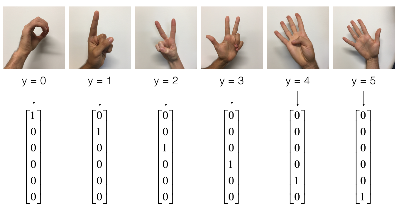
['/usr/local/lib/python3.6/dist-packages/tensorflow']运行下面的单元来加载数据集,它里面包含的是0到5的手势。
X_train_orig, Y_train_orig, X_test_orig, Y_test_orig, classes = load_dataset()
下面的单元会将数据集里面的某个样本的图片已经它对应的数字打印出来。你可以更改一下index的值,让它打印出不同的样本。
index = 6
plt.imshow(X_train_orig[index])
print ("y = " + str(np.squeeze(Y_train_orig[:, index])))
y = 2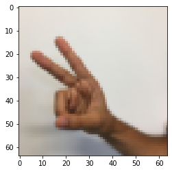
其实在第二章的时候,我们就已经接触了这个数据集。当时我们是在它上面构建了一个全链接神经网络。其实我们应该使用CNN,因为这些数据是图片。就如我们教程中所说的,只要提到智能视觉,那么就应该想到CNN。
下面我们先把这些数据的维度打印出来。因为编程中常常会出现因为维度错乱而导致bug出现。而且一旦出现了还很不好查,所以我们会在很多地方把维度信息打印出来。即可以防止出现维度错乱,又可以在出现bug后帮助定位问题。
X_train = X_train_orig/255.
X_test = X_test_orig/255.
Y_train = convert_to_one_hot(Y_train_orig, 6).T
Y_test = convert_to_one_hot(Y_test_orig, 6).T
print ("训练样本数 = " + str(X_train.shape[0]))
print ("测试样本数 = " + str(X_test.shape[0]))
print ("X_train的维度: " + str(X_train.shape))
print ("Y_train的维度: " + str(Y_train.shape))
print ("X_test的维度: " + str(X_test.shape))
print ("Y_test的维度: " + str(Y_test.shape))
conv_layers = {}
训练样本数 = 1080
测试样本数 = 120
X_train的维度: (1080, 64, 64, 3)
Y_train的维度: (1080, 6)
X_test的维度: (120, 64, 64, 3)
Y_test的维度: (120, 6)1.1 - 创建占位符(placeholders)
要使用TensorFlow,首先我们需要为训练数据准备好占位符,这样一来,在运行tensorflow session时我们就可以把数据填充到占位符中供TensorFlow使用。
下面的函数会为样本X和标签Y分别创建占位符。在代码中我们没有指定样本的数量,因为这样会使代码更加灵活,可以让我们在后面才决定样本数量。
def create_placeholders(n_H0, n_W0, n_C0, n_y):
    """
    参数:
    n_H0 -- 图像矩阵的高
    n_W0 -- 图像矩阵的宽
    n_C0 -- 图像矩阵的深度
    n_y -- 标签类别数量,我们的数据集是0到5的手势,所以有6个类别

    返回值:
    X -- 样本数据的占位符
    Y -- 标签的占位符
    """

    # 下面使用None来表示样本数量,表示当前还不确定样本数量
    X = tf.placeholder(tf.float32, [None, n_H0, n_W0, n_C0])
    Y = tf.placeholder(tf.float32, [None, n_y])

    return X, Y
X, Y = create_placeholders(64, 64, 3, 6)
print ("X = " + str(X))
print ("Y = " + str(Y))X = Tensor("Placeholder:0", shape=(?, 64, 64, 3), dtype=float32)
Y = Tensor("Placeholder_1:0", shape=(?, 6), dtype=float32)1.2 - 初始化参数
def initialize_parameters():

    tf.set_random_seed(1)

    #使用`tf.contrib.layers.xavier_initializer(seed = 0)`来初始化W1。
    # W1的维度是[4, 4, 3, 8],表示第一个卷积层过滤器矩阵的[高,宽,深度,个数]
    W1 = tf.get_variable("W1", [4, 4, 3, 8], initializer=tf.contrib.layers.xavier_initializer(seed=0))
    # W1 = tf.get_variable("W1", [4, 4, 3, 8], initializer=tf.truncated_normal_initializer(stddev=0.1))

    #初始化W2
    W2 = tf.get_variable("W2", [2, 2, 8, 16], initializer=tf.contrib.layers.xavier_initializer(seed=0))

    #有同学会问,为什么不初始化阈值和全连接层的相关参数呢?
    #因为TensorFlow会自动初始化它们,不需要我们操心

    parameters = {"W1": W1,
                  "W2": W2}

    return parameters
tf.reset_default_graph()
with tf.Session() as sess_test:
parameters = initialize_parameters()
init = tf.global_variables_initializer()
sess_test.run(init)
print("W1 = " + str(parameters["W1"].eval()[1,1,1]))
print("W2 = " + str(parameters["W2"].eval()[1,1,1]))W1 = [ 0.00131723 0.1417614 -0.04434952 0.09197326 0.14984085 -0.03514394
-0.06847463 0.05245192]
W2 = [-0.08566415 0.17750949 0.11974221 0.16773748 -0.0830943 -0.08058
-0.00577033 -0.14643836 0.24162132 -0.05857408 -0.19055021 0.1345228
-0.22779644 -0.1601823 -0.16117483 -0.10286498]1.2 - 前向传播
TensorFlow提供了一些CNN相关的工具函数。
-
tf.nn.conv2d(X,W1, strides = [1,s,s,1], padding = 'SAME'): X是指输入矩阵,W1是指过滤器。这个函数会将X和W1进行卷积。strides是指各个维度的卷积步长,[1,s,s,1]的含义分别是[样本数,输入矩阵的高,输入矩阵的宽,输入矩阵的深度]。padding是指填补数量,默认使用SAME填补,也就是自动填补一定数量元素而保证输入矩阵与输出矩阵的尺寸一样。
-
tf.nn.max_pool(A, ksize = [1,f,f,1], strides = [1,s,s,1], padding = 'SAME'): 这个函数会对输入矩阵A进行最大池化。ksize中的f表示池化窗口的大小。strides中的s表示步长。
-
tf.nn.relu(Z1): 对Z1中的每一个元素进行relu激活
-
tf.contrib.layers.flatten(P): 它会将P中样本的矩阵扁平化成向量。
-
tf.contrib.layers.fully_connected(F, num_outputs): 构建一个全连接层,F是该层的输入,num_outputs表示该层中神经元的个数。这个函数会自动初始化该层的权重w。我们在前面只初始化了卷积层相关的参数,因为TensorFlow会自动帮我们初始化全链接层的参数。
def forward_propagation(X, parameters):
    """
    这个函数会实现如下的前向传播流程:
    CONV2D卷积 -> RELU激活 -> MAXPOOL池化 -> CONV2D卷积 -> RELU激活 -> MAXPOOL池化 -> FLATTEN扁平化 -> 全连接层

    参数:
    X -- 输入特征的占位符
    parameters -- 之前我们初始化好的"W1", "W2"参数

    Returns:
    Z3 -- 最后一个全连接层的输出
    """

    W1 = parameters['W1']
    W2 = parameters['W2']

    Z1 = tf.nn.conv2d(X, W1, strides=[1, 1, 1, 1], padding='SAME')

    A1 = tf.nn.relu(Z1)

    P1 = tf.nn.max_pool(A1, ksize = [1, 8, 8, 1], strides = [1, 8, 8, 1], padding='SAME')

    Z2 = tf.nn.conv2d(P1, W2, strides=[1, 1, 1, 1], padding='SAME')

    A2 = tf.nn.relu(Z2)

    P2 = tf.nn.max_pool(A2, ksize = [1, 4, 4, 1], strides = [1, 4, 4, 1], padding='SAME')

    # @see doc https://tensorflow.google.cn/guide/migrate
    P = tf.contrib.layers.flatten(P2)

    # 指定该全连接层有6个神经元。
    # activation_fn=None表示该层没有激活函数,因为后面我们会再接一个softmax层
    Z3 = tf.contrib.layers.fully_connected(P, 6, activation_fn=None)

    return Z3
tf.reset_default_graph()
with tf.Session() as sess:
np.random.seed(1)
X, Y = create_placeholders(64, 64, 3, 6)
parameters = initialize_parameters()
Z3 = forward_propagation(X, parameters)
init = tf.global_variables_initializer()
sess.run(init)
a = sess.run(Z3, {X: np.random.randn(2,64,64,3), Y: np.random.randn(2,6)})
print("Z3 = " + str(a))Z3 = [[-0.44670227 -1.5720876 -1.5304923 -2.3101304 -1.2910438 0.46852064]
[-0.17601591 -1.5797201 -1.4737016 -2.616721 -1.0081065 0.5747785 ]]1.3 - 计算损失
def compute_cost(Z3, Y):
    """
    参数:
    Z3 -- 前面forward_propagation的输出结果,维度是(6, 样本数)
    Y -- 真实标签的占位符,维度当然也是(6, 样本数)

    返回值:
    cost - 返回一个tensorflow张量,它代表了softmax激活以及成本计算操作。
    """

    # tf.nn.softmax_cross_entropy_with_logits函数不仅仅执行了softmax激活,还将成本也给计算了。
    # tf.reduce_mean本用来获取平均值。在这里被用于获取多个样本的平均损失,即获取成本。
    cost = tf.reduce_mean(tf.nn.softmax_cross_entropy_with_logits(logits=Z3, labels=Y))

    return cost
tf.reset_default_graph()
with tf.Session() as sess:
np.random.seed(1)
X, Y = create_placeholders(64, 64, 3, 6)
parameters = initialize_parameters()
Z3 = forward_propagation(X, parameters)
cost = compute_cost(Z3, Y)
init = tf.global_variables_initializer()
sess.run(init)
a = sess.run(cost, {X: np.random.randn(4,64,64,3), Y: np.random.randn(4,6)})
print("cost = " + str(a))cost = 2.91033961.4 构建模型
最终,我们将上面那些工具函数组合起来,构建一个CNN网络模型。并且用手势数据集来训练它。
def model(X_train, Y_train, X_test, Y_test, learning_rate=0.009,
          num_epochs=100, minibatch_size=64, print_cost=True):
    """
    参数:
    X_train -- 训练集数据,维度是(1080, 64, 64, 3)
    Y_train -- 训练集标签, 维度是(1080, 6)
    X_test -- 测试集数据, 维度是(120, 64, 64, 3)
    Y_test -- 测试集标签, 维度是(120, 6)

    返回值:
    train_accuracy -- 训练集上的预测精准度
    test_accuracy -- 测试集上的预测精准度
    parameters -- 训练好的参数
    """

    ops.reset_default_graph()                         # 重置一下tf框架
    tf.set_random_seed(1)
    seed = 3
    (m, n_H0, n_W0, n_C0) = X_train.shape
    n_y = Y_train.shape[1]   # n_y是标签的类别数量,这里是6
    costs = []

    X, Y = create_placeholders(n_H0, n_W0, n_C0, n_y)

    parameters = initialize_parameters()

    Z3 = forward_propagation(X, parameters)

    cost = compute_cost(Z3, Y)

    # 我们使用adam来作为优化算法
    optimizer = tf.train.AdamOptimizer(learning_rate=learning_rate).minimize(cost)

    init = tf.global_variables_initializer()

    with tf.Session() as sess:

        sess.run(init)

        for epoch in range(num_epochs):

            minibatch_cost = 0.
            num_minibatches = int(m / minibatch_size)
            seed = seed + 1
            minibatches = random_mini_batches(X_train, Y_train, minibatch_size, seed)

            for minibatch in minibatches:

                (minibatch_X, minibatch_Y) = minibatch
                # 执行session。训练正式开始。每一次训练一个子训练集minibatch
                _ , temp_cost = sess.run([optimizer, cost], feed_dict={X:minibatch_X, Y:minibatch_Y})

                minibatch_cost += temp_cost / num_minibatches

            if print_cost == True and epoch % 5 == 0:
                print ("Cost after epoch %i: %f" % (epoch, minibatch_cost))
            if print_cost == True and epoch % 1 == 0:
                costs.append(minibatch_cost)

        plt.plot(np.squeeze(costs))
        plt.ylabel('cost')
        plt.xlabel('iterations (per tens)')
        plt.title("Learning rate =" + str(learning_rate))
        plt.show()

        # 计算预测精准度
        predict_op = tf.argmax(Z3, 1)
        correct_prediction = tf.equal(predict_op, tf.argmax(Y, 1))
        accuracy = tf.reduce_mean(tf.cast(correct_prediction, "float"))
        print(accuracy)
        train_accuracy = accuracy.eval({X: X_train, Y: Y_train})
        test_accuracy = accuracy.eval({X: X_test, Y: Y_test})
        print("训练集预测精准度:", train_accuracy)
        print("测试集预测精准度:", test_accuracy)

        return train_accuracy, test_accuracy, parameters
_, _, parameters = model(X_train, Y_train, X_test, Y_test)Cost after epoch 0: 1.917929
Cost after epoch 5: 1.506757
Cost after epoch 10: 0.955359
Cost after epoch 15: 0.845802
Cost after epoch 20: 0.701174
Cost after epoch 25: 0.572085
Cost after epoch 30: 0.521668
Cost after epoch 35: 0.532902
Cost after epoch 40: 0.431018
Cost after epoch 45: 0.401331
Cost after epoch 50: 0.370733
Cost after epoch 55: 0.365420
Cost after epoch 60: 0.283705
Cost after epoch 65: 0.323672
Cost after epoch 70: 0.307099
Cost after epoch 75: 0.294215
Cost after epoch 80: 0.273980
Cost after epoch 85: 0.243726
Cost after epoch 90: 0.242174
Cost after epoch 95: 0.191030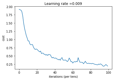
Tensor("Mean_1:0", shape=(), dtype=float32)
训练集预测精准度: 0.9138889
测试集预测精准度: 0.7916667
预测精准度有可能会上下浮动一点点。
恭喜!我们一起构建了一个可以识别手语CNN程序,识别率达到了75%左右。当然,你还可以继续提升它,通过微调超参数,以及使用我们在第3章中学到的知识来分析优化它。
坚持跟我学到了现在,值得表扬,给你个大拇指!去逛逛pornhub放松放松吧!
# 预测图片
fname = "images/test_up_1.jpeg"
image = np.array(plt.imread(fname))
my_image = scipy.misc.imresize(image, size=(64,64))
plt.imshow(my_image)

#print(parameters)
#my_image_prediction = predict(my_image, parameters)

#print("Your algorithm predicts: y = " + str(np.squeeze(my_image_prediction)))
/usr/local/lib/python3.6/dist-packages/ipykernel_launcher.py:4: DeprecationWarning: `imresize` is deprecated!
`imresize` is deprecated in SciPy 1.0.0, and will be removed in 1.3.0.
Use Pillow instead: ``numpy.array(Image.fromarray(arr).resize())``.
after removing the cwd from sys.path.
<matplotlib.image.AxesImage at 0x7f2b585bcac8>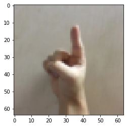
辅助函数
cnn_utils.py
import math
import numpy as np
import h5py
import matplotlib.pyplot as plt
import tensorflow as tf
#import tensorflow.compat.v1 as tf # 这里使用V1版本
#tf.disable_v2_behavior() # # 关掉 v2 版本
#from tensorflow.python.framework import ops

def load_dataset():
    train_dataset = h5py.File('datasets/train_signs.h5', "r")
    train_set_x_orig = np.array(train_dataset["train_set_x"][:]) # your train set features
    train_set_y_orig = np.array(train_dataset["train_set_y"][:]) # your train set labels

    test_dataset = h5py.File('datasets/test_signs.h5', "r")
    test_set_x_orig = np.array(test_dataset["test_set_x"][:]) # your test set features
    test_set_y_orig = np.array(test_dataset["test_set_y"][:]) # your test set labels

    classes = np.array(test_dataset["list_classes"][:]) # the list of classes

    train_set_y_orig = train_set_y_orig.reshape((1, train_set_y_orig.shape[0]))
    test_set_y_orig = test_set_y_orig.reshape((1, test_set_y_orig.shape[0]))

    return train_set_x_orig, train_set_y_orig, test_set_x_orig, test_set_y_orig, classes

def random_mini_batches(X, Y, mini_batch_size = 64, seed = 0):
    """
    Creates a list of random minibatches from (X, Y)

    Arguments:
    X -- input data, of shape (input size, number of examples) (m, Hi, Wi, Ci)
    Y -- true "label" vector (containing 0 if cat, 1 if non-cat), of shape (1, number of examples) (m, n_y)
    mini_batch_size - size of the mini-batches, integer
    seed -- this is only for the purpose of grading, so that you're "random minibatches are the same as ours.

    Returns:
    mini_batches -- list of synchronous (mini_batch_X, mini_batch_Y)
    """

    m = X.shape[0]                  # number of training examples
    mini_batches = []
    np.random.seed(seed)

    # Step 1: Shuffle (X, Y)
    permutation = list(np.random.permutation(m))
    shuffled_X = X[permutation,:,:,:]
    shuffled_Y = Y[permutation,:]

    # Step 2: Partition (shuffled_X, shuffled_Y). Minus the end case.
    num_complete_minibatches = math.floor(m/mini_batch_size) # number of mini batches of size mini_batch_size in your partitionning
    for k in range(0, num_complete_minibatches):
        mini_batch_X = shuffled_X[k * mini_batch_size : k * mini_batch_size + mini_batch_size,:,:,:]
        mini_batch_Y = shuffled_Y[k * mini_batch_size : k * mini_batch_size + mini_batch_size,:]
        mini_batch = (mini_batch_X, mini_batch_Y)
        mini_batches.append(mini_batch)

    # Handling the end case (last mini-batch < mini_batch_size)
    if m % mini_batch_size != 0:
        mini_batch_X = shuffled_X[num_complete_minibatches * mini_batch_size : m,:,:,:]
        mini_batch_Y = shuffled_Y[num_complete_minibatches * mini_batch_size : m,:]
        mini_batch = (mini_batch_X, mini_batch_Y)
        mini_batches.append(mini_batch)

    return mini_batches

def convert_to_one_hot(Y, C):
    Y = np.eye(C)[Y.reshape(-1)].T
    return Y

def forward_propagation_for_predict(X, parameters):
    """
    Implements the forward propagation for the model: LINEAR -> RELU -> LINEAR -> RELU -> LINEAR -> SOFTMAX

    Arguments:
    X -- input dataset placeholder, of shape (input size, number of examples)
    parameters -- python dictionary containing your parameters "W1", "b1", "W2", "b2", "W3", "b3"
                  the shapes are given in initialize_parameters

    Returns:
    Z3 -- the output of the last LINEAR unit
    """

    # Retrieve the parameters from the dictionary "parameters"
    W1 = parameters['W1']
    b1 = parameters['b1']
    W2 = parameters['W2']
    b2 = parameters['b2']
    W3 = parameters['W3']
    b3 = parameters['b3']
                                                           # Numpy Equivalents:
    Z1 = tf.add(tf.matmul(W1, X), b1)                      # Z1 = np.dot(W1, X) + b1
    A1 = tf.nn.relu(Z1)                                    # A1 = relu(Z1)
    Z2 = tf.add(tf.matmul(W2, A1), b2)                     # Z2 = np.dot(W2, a1) + b2
    A2 = tf.nn.relu(Z2)                                    # A2 = relu(Z2)
    Z3 = tf.add(tf.matmul(W3, A2), b3)                     # Z3 = np.dot(W3,Z2) + b3

    return Z3

def predict(X, parameters):

    W1 = tf.convert_to_tensor(parameters["W1"])
    b1 = tf.convert_to_tensor(parameters["b1"])
    W2 = tf.convert_to_tensor(parameters["W2"])
    b2 = tf.convert_to_tensor(parameters["b2"])
    W3 = tf.convert_to_tensor(parameters["W3"])
    b3 = tf.convert_to_tensor(parameters["b3"])

    params = {"W1": W1,
              "b1": b1,
              "W2": W2,
              "b2": b2,
              "W3": W3,
              "b3": b3}

    x = tf.placeholder("float", [12288, 1])

    z3 = forward_propagation_for_predict(x, params)
    p = tf.argmax(z3)

    sess = tf.Session()
    prediction = sess.run(p, feed_dict = {x: X})

    return prediction

#def predict(X, parameters):
#
#    W1 = tf.convert_to_tensor(parameters["W1"])
#    b1 = tf.convert_to_tensor(parameters["b1"])
#    W2 = tf.convert_to_tensor(parameters["W2"])
#    b2 = tf.convert_to_tensor(parameters["b2"])
##    W3 = tf.convert_to_tensor(parameters["W3"])
##    b3 = tf.convert_to_tensor(parameters["b3"])
#
##    params = {"W1": W1,
##              "b1": b1,
##              "W2": W2,
##              "b2": b2,
##              "W3": W3,
##              "b3": b3}
#
#    params = {"W1": W1,
#              "b1": b1,
#              "W2": W2,
#              "b2": b2}
#
#    x = tf.placeholder("float", [12288, 1])
#
#    z3 = forward_propagation(x, params)
#    p = tf.argmax(z3)
#
#    with tf.Session() as sess:
#        prediction = sess.run(p, feed_dict = {x: X})
#
#    return prediction
为者常成,行者常至
自由转载-非商用-非衍生-保持署名(创意共享3.0许可证)


