
Python:matplotlib 之直方图 (二十八)
直方图
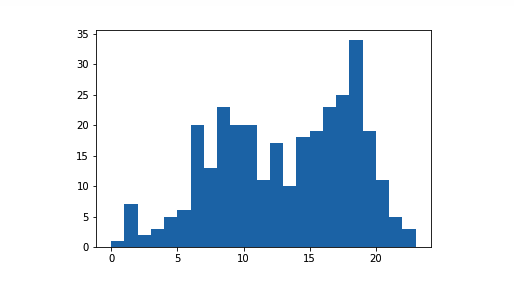
直方图用来绘制数字变量的分布情况。它是条形图的定量版本。但是,我们不再为每个独特数字值绘制一个长条,而是将值分成连续的分箱,并针对每个分箱绘制一个长条,用于描绘相关数字。例如,使用 matplotlib 的 hist 函数的默认设置:
plt.hist(data = df, x = 'num_var')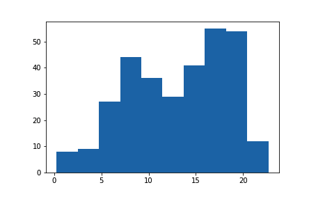
可以看出,在最左侧的分箱(约为 0 到 2.5 之间)中有 8 个数据点,在相邻分箱(约为 2.5 到 5 之间)中有 9 个数据点。总体来说,可以看出是一个双峰分布。直方图中的长条直接相连,而条形图中的长条是分开的,表明在直方图中数据的值处在连续范围内。如果某个数据值位于分箱边缘,则属于右侧分箱。例外情况是最右侧的分箱边缘,将上限的值放入最右侧的分箱内(上限的左侧)。
默认情况下,hist 函数会根据值的范围将数据分成 10 个分箱。在几乎所有情况下,我们都需要更改这一设置。通常,只有 10 个分箱太少了,无法了解数据的分布情况。并且默认的刻度并没有采用很容易解释分箱范围的近似值。如果在上述示例中,将“约为 0 到 2.5 之间”说成“0 到 2.5 之间”并将“约为 2.5 到 5 之间”说成“2.5 到 5 之间”,是不是更方便?
你可以使用描述统计学(例如通过 df['num_var'].describe())估测什么样的分箱下限和分箱上限比较合适。可以使用 numpy 的 arange 函数设置这些分箱边缘:
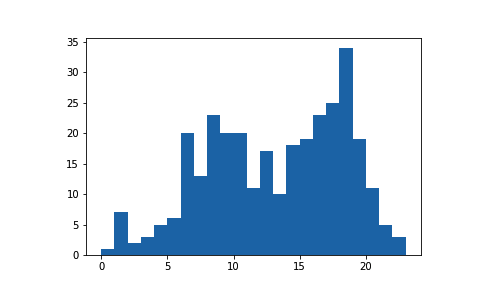
bin_edges = np.arange(0, df['num_var'].max()+1, 1)
plt.hist(data = df, x = 'num_var', bins = bin_edges)
arange 的第一个参数是最左侧的分箱边缘,第二个参数是上限,第三个参数是分箱宽度。注意,即使我在第二个参数中指定了“max”值,我添加了“+1”(分箱宽度)。这是因为 arange 将仅返回完全小于上限的值。加上“+1”可有效地确保左右侧的分箱边缘至少是最大数据值,以便所有数据点都能绘制出来。最左侧的分箱设为硬编码的值,以便获得可解释的值,当然你也可以使用 numpy 的 around 等函数以程序方式达到这种效果。
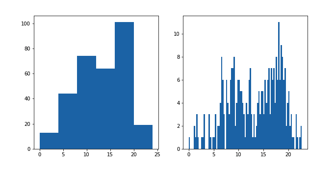
在创建直方图时,有必要尝试不同的分箱宽度,看看哪个宽度最能表示数据。如果分箱太多,可能会发现太多噪点,干扰我们发现数据蕴含的规律。如果分箱太少,则根本无法看出真正的规律。
plt.figure(figsize = [10, 5]) # larger figure size for subplots

# histogram on left, example of too-large bin size
plt.subplot(1, 2, 1) # 1 row, 2 cols, subplot 1
bin_edges = np.arange(0, df['num_var'].max()+4, 4)
plt.hist(data = df, x = 'num_var', bins = bin_edges)

# histogram on right, example of too-small bin size
plt.subplot(1, 2, 2) # 1 row, 2 cols, subplot 2
bin_edges = np.arange(0, df['num_var'].max()+1/4, 1/4)
plt.hist(data = df, x = 'num_var', bins = bin_edges)
该示例通过 subplot 函数将两个图形并排地放到一起,函数的参数指定了有效子图的行数、列数和索引。figure()函数在调用时传入了 "figsize" 参数,以便我们能够绘制更大的图形并包含多个子图。
替代方法
seaborn 函数 distplot也可以用于绘制直方图,并且与其他单变量绘图函数集成到一起。
sb.distplot(df['num_var'])注意,第一个参数_必须_是 Series 或数组,其中包含要绘制的数据点,而不是指定数据来源和列。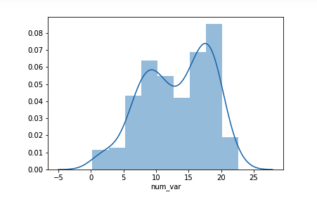
distplot 函数具有指定直方图分箱的内置规则,默认情况下,会在数据上方绘制一个 (KDE) 核密度估计。纵轴基于 KDE,而不是直方图:长条的高度之和不一定等于 1,但是曲线下方的面积应该等于 1。如果你想详细了解 KDE,请参阅这节课末尾的补充内容。
虽然默认的 distplot分箱尺寸可能比固定的 .hist = 10 更合适,但是你依然需要进行调整,使分箱尺寸等于四舍五入的值。你可以使用其他参数设置绘制直方图并像之前一样指定分箱:
bin_edges = np.arange(0, df['num_var'].max()+1, 1)
sb.distplot(df['num_var'], bins = bin_edges, kde = False,
            hist_kws = {'alpha' : 1})
alpha(透明度)设置必须当做字典与 "hist_kws" 关联,因为还有其他底层绘图函数(例如 KDE)具有自己的可选关键字参数。
上述代码的结果和上述分箱宽度为 1 的直方图完全一样。纵轴的单位也以计数的形式出现了。
直方图练习
# prerequisite package imports
import numpy as np
import pandas as pd
import matplotlib.pyplot as plt
import seaborn as sb

%matplotlib inline

from solutions_univ import histogram_solution_1
在此 workspace 中,我们将继续使用 Pokémon 数据集。
pokemon = pd.read_csv('./data/pokemon.csv')
pokemon.head()| id | species | generation_id | height | weight | base_experience | type_1 | type_2 | hp | attack | defense | speed | special-attack | special-defense | |
|---|---|---|---|---|---|---|---|---|---|---|---|---|---|---|
| 0 | 1 | bulbasaur | 1 | 0.7 | 6.9 | 64 | grass | poison | 45 | 49 | 49 | 45 | 65 | 65 |
| 1 | 2 | ivysaur | 1 | 1.0 | 13.0 | 142 | grass | poison | 60 | 62 | 63 | 60 | 80 | 80 |
| 2 | 3 | venusaur | 1 | 2.0 | 100.0 | 236 | grass | poison | 80 | 82 | 83 | 80 | 100 | 100 |
| 3 | 4 | charmander | 1 | 0.6 | 8.5 | 62 | fire | NaN | 39 | 52 | 43 | 65 | 60 | 50 |
| 4 | 5 | charmeleon | 1 | 1.1 | 19.0 | 142 | fire | NaN | 58 | 64 | 58 | 80 | 80 | 65 |
任务:Pokémon 具有很多描述作战能力的统计指标。在此任务中,请创建一个直方图,用于描绘 'special-defense' 值的分布情况。提示:请尝试不同的分箱宽度大小,看看哪个大小最适合描绘数据。
# YOUR CODE HERE
# 1.简单的直方图
# plt.hist(data=pokemon, x='special-defense')

# 2.使用 numpy 的 arange 函数设置这些分箱边缘
bin_edges = np.arange(0, pokemon['special-defense'].max() + 10, 10)
print(bin_edges)
plt.hist(data=pokemon, x='special-defense', bins=bin_edges)
[ 0 10 20 30 40 50 60 70 80 90 100 110 120 130 140 150 160 170
180 190 200 210 220 230]
(array([ 0., 0., 18., 57., 102., 125., 116., 108., 94.,
71., 47., 25., 14., 16., 3., 9., 0., 0.,
0., 0., 1., 0., 1.]),
array([ 0, 10, 20, 30, 40, 50, 60, 70, 80, 90, 100, 110, 120,
130, 140, 150, 160, 170, 180, 190, 200, 210, 220, 230]),
<a list of 23 Patch objects>)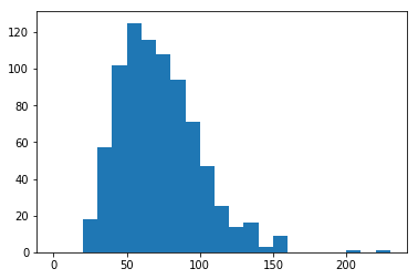
# run this cell to check your work against ours
histogram_solution_1()
I've used matplotlib's hist function to plot the data. I have also used numpy's arange function to set the bin edges. A bin size of 5 hits the main cut points, revealing a smooth, but skewed curves. Are there similar characteristics among Pokemon with the highest special defenses?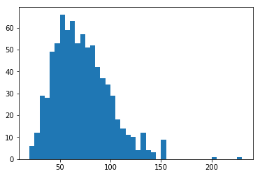
bin_edges = np.arange(0, pokemon['special-defense'].max()+5, 5)
sb.distplot(pokemon['special-defense'], bins = bin_edges, kde = True,
            hist_kws = {'alpha' : 1})
<matplotlib.axes._subplots.AxesSubplot at 0x7f3f8536bdd8>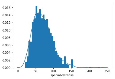
为者常成,行者常至
自由转载-非商用-非衍生-保持署名(创意共享3.0许可证)


